Pipe analysis
MetaPiping proposes a detailed analysis of pipe.
After piping analysis, the pipes can be examined.
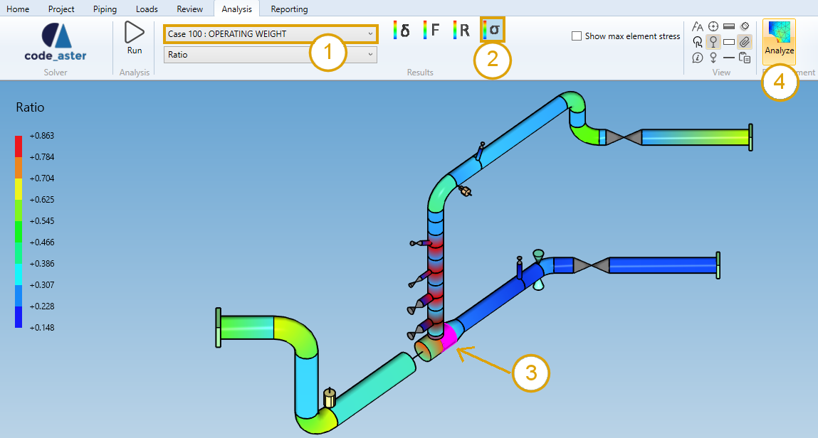
- Select a load case or mode (1).
- Select the stress button (2).
- Select either a pipe in the 3D space or in the results table (3).
- Click on the Analysis button (4).
The selection mode is automatically set to Element when clicking on stress button.
1. Template
You can then choose a template of Finite element :
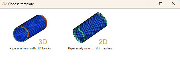
- 3D bricks : second order 20-node hexahedrons for curved volumetric element
- 2D meshes : second order 8-node quadrangles for curved surface element
If other analysis exists for the same Element, the same Load and the same Template, a window will appear :
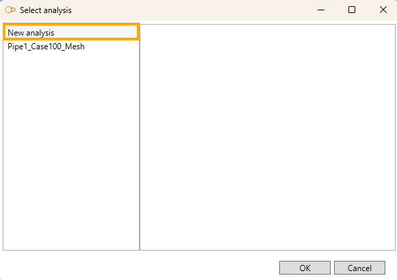
- Select New analysis to start a new analysis from scratch.
- Or select an existing analysis to reopen it :
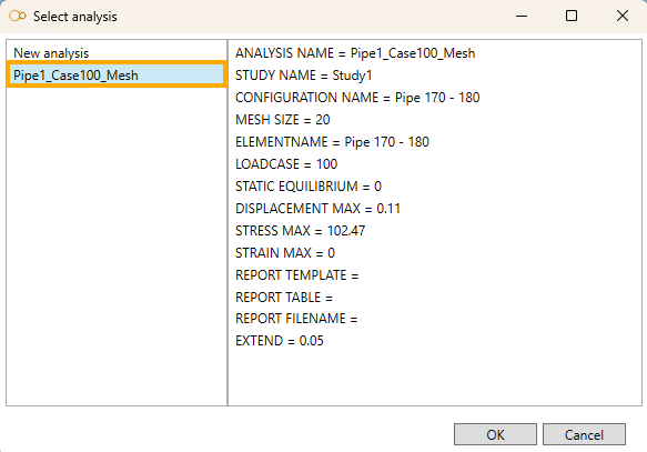
Some properties and results are shown.
Click OK.
2. New analysis
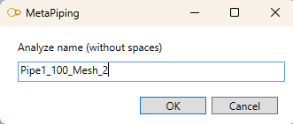
If you choose to create a New analysis, you have to define a name to the analysis (that doesn’t already exist) :
The Finite Element Analysis Window appears (2D mesh template) :
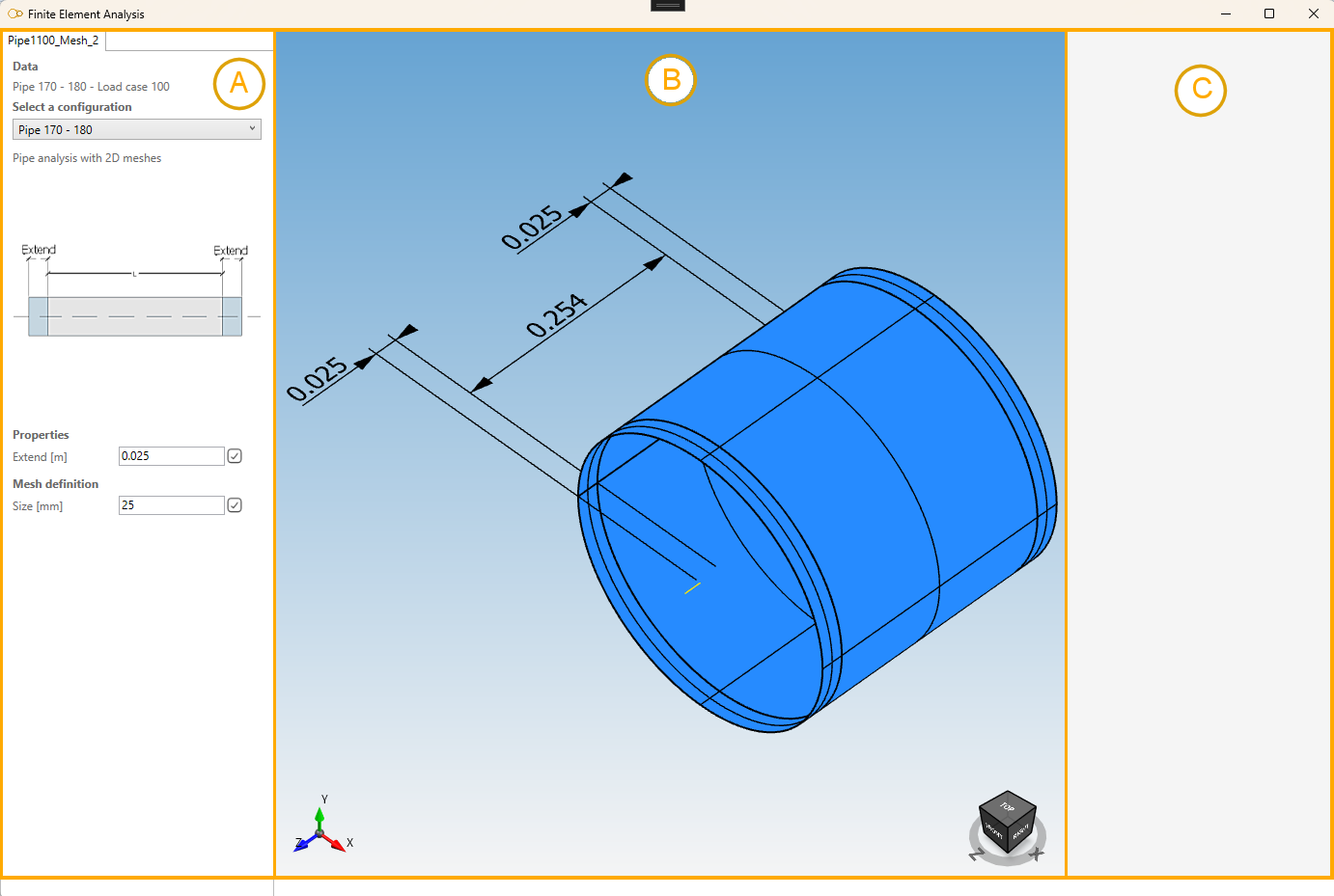
MetaPiping automatically transforms the actual pipe to surfacing elements (on neutral fiber).
The window is divided into 3 areas :
- A : Definition of the assembly, mesh, results and report
- B : Model 3D
- C : Groups of elements with same properties (type, thickness, material)
The first area contains 1 geometric property and 1 mesh property :
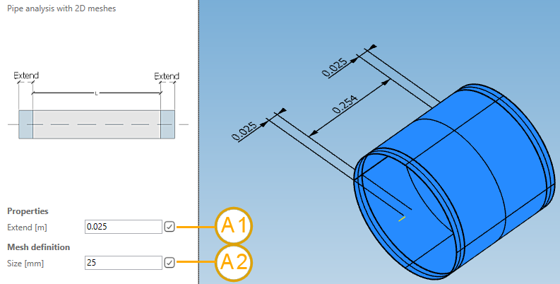
- A1 : The length of extend. Click on v button to modify.
- A2 : The desired mesh size. Click on v button to generate the meshing.
Set for example 0.05 m of extend and a mesh size of 20 mm.
3. Meshing
Choose a mesh size and click on v button (1) :
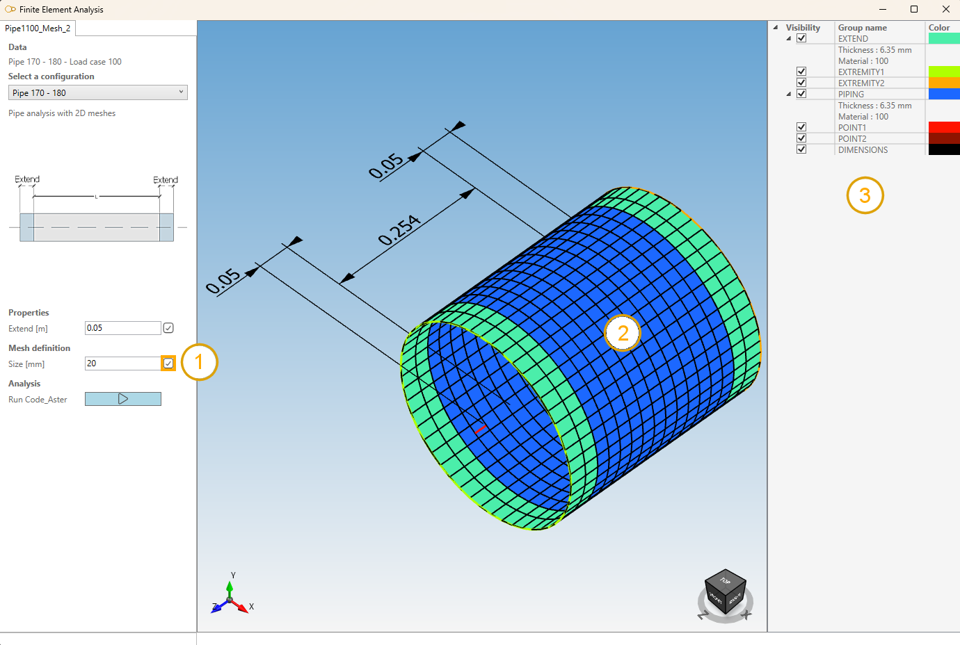
After several seconds, the assembly is totally meshed (2).
All groups appears on the right (3). You can show/hide each group for a better visualization.
The Code_Aster button is now available for a complete calculation.
4. Finite element analysis
Click on the Code_Aster button to launch a detailed calculation (1) :
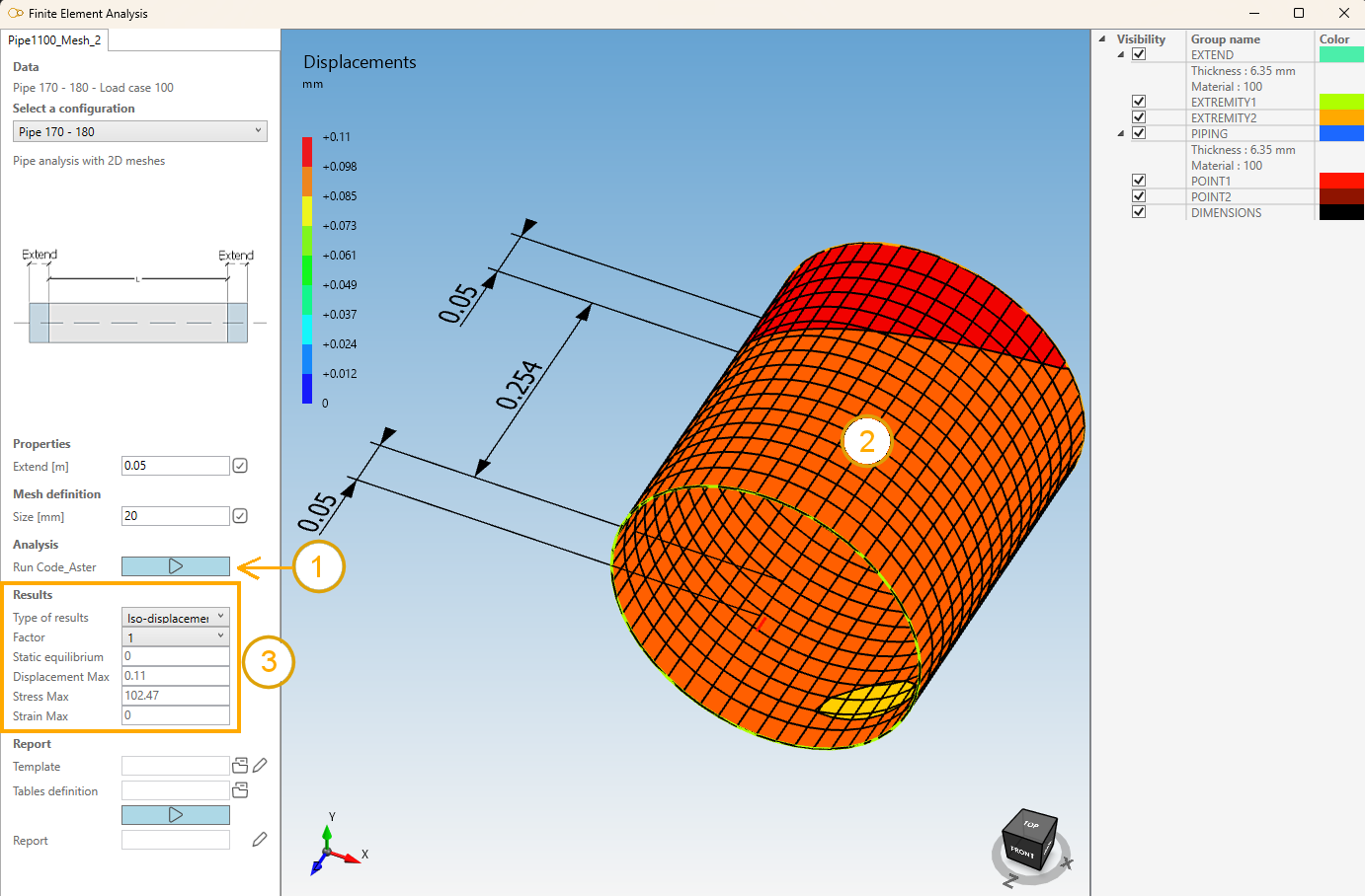
Colored results appears (2) with a corresponding legend.
A result panel appears where the type of results can be choose and some informations are shown (3).
Type of results :
| Property | Unit Metric | Unit USA | Remark |
|---|---|---|---|
| Groups | - | - | |
| Displacements | mm | in | Use Factor to amplify the deformation |
| Stresses | N/mm² | ksi | |
| Strains | % | % | |
| Iso-displacements | mm | in | Use Factor to amplify the deformation |
| Iso-stresses | N/mm² | ksi | |
| Iso-Strains | % | % |
The Static equilibrium is also evaluated (value near 0 reaches the perfect equilibrium).
Static Equilibrium refers to the physical state in which a system is at rest and the net force acting
on it is null. It is a state in which all the forces acting on an object are balanced out and the
object is not found to be in motion to the relative plane.
5. Report
A report can be generated based on a template and “tables” file.
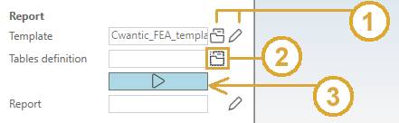
- Select a template (open button) or edit template (pencil button) (1).
- Select a tables file (open button) (2).
- Click on the Report button to generate the report (3).
Use the default template Cwantic_FEA_Piping_template_SI
The template is copy from the settings to the analysis’ directory and can be locally modified before report generation (requires Microsoft Word).
The select document window (example for table) :
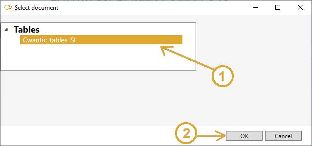
- Select the document (1)
- Click OK (2)
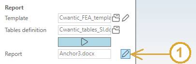
After generation, the report receive the name of the analysis.
You can edit the final report by clicking on the pencil button (requires Microsoft Word) (1) :
Click here to have more information about the reporting mechanism.
5.1 Keywords
The keyword is useful to make a correspondence between the template and the table document but with specific decorators :
$$keyword$$ for the template
[keyword] for the table
| Keyword | Description | Remark |
|---|---|---|
| STUDY NAME | The name of the current study | No table |
| ANALYSIS NAME | The name of the current analysis | No table |
| PICTURE | Take a picture (§5.2) | No table |
| CONFIG PICTURE | The picture of the current config | No table |
| MESH RESULTS | The list of all mesh results | table [MESH RESULTS] |
| CONFIGURATION NAME | The name of the current configuration | No table |
| ELEMENT PROPERTIES | The element properties | table [ELEMENT PROPERTIES] |
| MESH SIZE | The meshing properties | table [MESH SIZE] |
| ELEMENTNAME | The name of the current element | No table |
| LOADCASE | The current load case | No table |
| STATIC EQUILIBRIUM | The static equilibrium value | No table |
| DISPLACEMENT MAX | The displacement max | No table |
| STRESS MAX | The stress max | No table |
| STRAIN MAX | The strain max | No table |
| FASTENER RATIO MAX | The max ratio on all fasteners | No table |
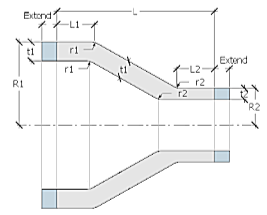
CONFIG PICTURE for pipe =
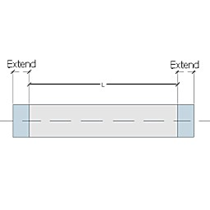
CONFIG PICTURE for bend =
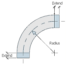
CONFIG PICTURE for concentric reducer =
5.2 Picture
It is possible to include pictures in the report with use of the keyword PICTURE.
When the software encounters this keyword, it simply makes a screenshot of the 3D engine.
It is possible to change the kind of visualization via a JSON structure just after the keyword separated by a semicolon character :
$$PICTURE;{...}$$
JSON parameters :
| Parameter | Description | Default value |
|---|---|---|
| Groups | An array of visible group name | Empty list = all groups will be visible |
| View | Orientation of the camera | 35 (= FrontFaceTopLeft - see below) |
| ResultType | Result category | 0 (= Group - see below) |
| Factor | Amplification factor of the displacements | 1 |
| Dim | 1 = show dimensions | 1 |
View values :
    Front                   = 0
    Right                   = 1
    Rear                    = 2
    Left                    = 3
    Top                     = 4
    Bottom                  = 5
    Isometric               = 6
    Dimetric                = 7
    Trimetric               = 8
    FrontFaceBottom         = 9
    FrontFaceRight          = 10
    FrontFaceTop            = 11
    FrontFaceLeft           = 12
    RightFaceBottom         = 13
    RightFaceRight          = 14
    RightFaceTop            = 15
    RightFaceLeft           = 16
    BackFaceBottom          = 17
    BackFaceRight           = 18
    BackFaceTop             = 19
    BackFaceLeft            = 20
    LeftFaceBottom          = 21
    LeftFaceRight           = 22
    LeftFaceTop             = 23
    LeftFaceLeft            = 24
    BottomFaceBottom        = 25
    BottomFaceRight         = 26
    BottomFaceTop           = 27
    BottomFaceLeft          = 28
    TopFaceBottom           = 29
    TopFaceRight            = 30
    TopFaceTop              = 31
    TopFaceLeft             = 32
    FrontFaceBottomLeft     = 33
    FrontFaceBottomRight    = 34
    FrontFaceTopLeft        = 35
    FrontFaceTopRight       = 36
    BackFaceBottomLeft      = 37
    BackFaceBottomRight     = 38
    BackFaceTopLeft         = 39
    BackFaceTopRight        = 40
Result type values :
    Group = 0
    Displacement = 1
    Stress = 2
    Strain = 3
    Compression = 4
    IsoDisplacement = 5
    IsoStress = 6
    IsoStrain = 7
    IsoCompression = 8
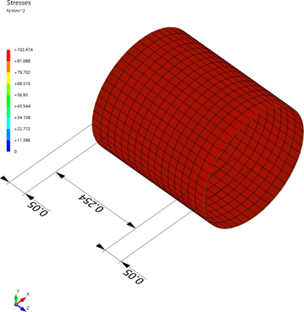
Example :
$$PICTURE;{“ResultType”:2,”View”:35,”Dim”:1}$$
ResultType = 2 for a “Stress” view
View = 35 for a FrontFaceTopLeft view
Dim = 1 will show the dimensions
Result :
6. Brick template
If you select the Brick template, some features change :
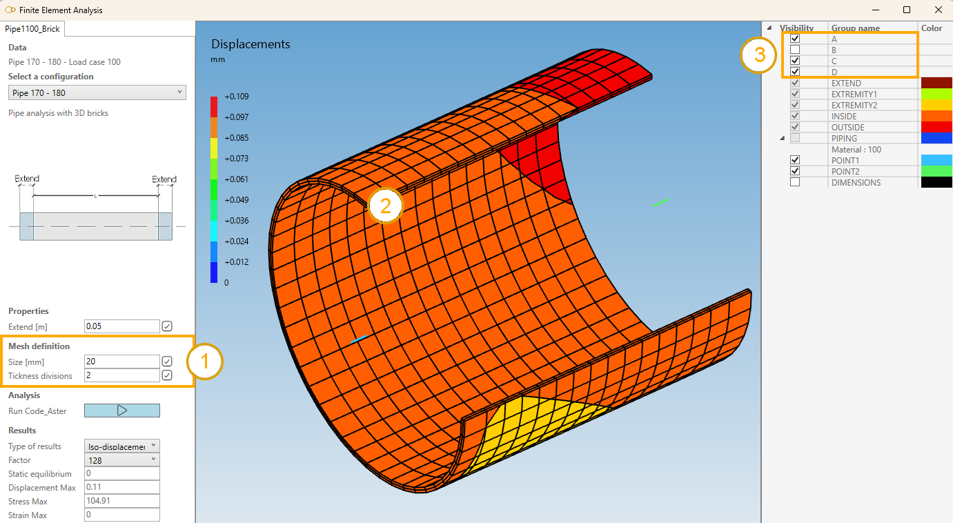
The mesh definition contains also the thickness division (= number of element in the thickness) and 4 groups that enable to hide part of the assembly (A, B, C and D).
In this example, you can see (2) a thickness division = 2 (1) and group B hidden to see the interior of the element.
7. Conclusion
The analysis is terminated.
You can keep this analysis on disk by closing the window and answer Yes to the question :
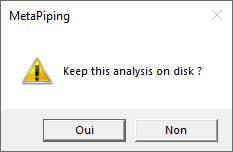
This analysis will be proposed on the window of §1 for the same element, load and template.